August 10, 2026

Quadratically-Constrained Quadratic Programming, Strong Duality, and the S-Lemma

In this post we are going to look at quadratically-constrained quadratic programs (QCQPs). In particular, we will examine the interesting result that strong duality holds (in most cases) for QCQPs with a single constraint, even when the problem is not convex. We made use of this fact previously when we looked at the convexity of the maximum eigenvalue of a symmetric matrix, and it is useful in many other areas like trust region optimization and control theory. This post is quite technical and assumes some familiarity with convex optimization; the standard (and freely available online) reference is Convex Optimization by Boyd and Vandenberghe.

Quadratically-Constrained Quadratic Programs

A general QCQP is an optimization problem with the form

\begin{equation}\label{1} \begin{aligned} p^{\star} = \min_{\bm{x}\in\mathbb{R}^n} &\quad f_0(\bm{x}) \\ \text{subject to} &\quad f_i(\bm{x}) \leq 0, \quad i=1,\dots,m, \end{aligned} \end{equation}

where

\begin{equation}\label{2} \begin{aligned} f_i(\bm{x}) &= \bm{x}^T\bm{Q}_i\bm{x} + 2\bm{p}_i^T\bm{x} + r_i \\ &= \begin{bmatrix} \bm{x} \\ 1 \end{bmatrix}^T\begin{bmatrix} \bm{Q}_i & \bm{p}_i \\ \bm{p}_i^T & r_i \end{bmatrix}\begin{bmatrix} \bm{x} \\ 1 \end{bmatrix} \end{aligned} \end{equation}

is a quadratic function with $\bm{Q}_i=\bm{Q}_i^T\in\mathbb{R}^{n\times n}$ , $\bm{p}_i\in\mathbb{R}^n$ , and $r_i\in\mathbb{R}$ for all $i=0,\dots,m$ . The form shown in the second line of $\eqref{2}$ is called the homogeneous form of $f_i$ . If $\bm{Q}_i\succcurlyeq\bm{0}$ (that is, $\bm{Q}_i$ is positive semidefinite), then $f_i$ is convex. If $f_i$ is convex for all $i=0,\dots,m$ , then $\eqref{1}$ is a convex problem; however, we are interested in the general case when we need not make such convexity assumptions. Note that quadratic equality constraints (which are always non-convex if $\bm{Q}_i\neq\bm{0}$ ) can be represented in $\eqref{1}$ as two-sided inequalities.

Many interesting problems in robotics can be expressed as QCQPs. Notably, the set of valid 3D rotations can be defined using non-convex quadratic constraints, allowing various state estimation problems to be cast as QCQPs. See e.g. (Holmes & Barfoot, 2023) for more information and examples.

Dual Problem

Let’s derive the (Lagrangian) dual problem of $\eqref{1}$ , roughly following Section 3.2 of (Park & Boyd, 2017). (We will refer to $\eqref{1}$ as the primal problem going forward.) The Lagrangian of $\eqref{1}$ is

\begin{equation}\label{3} \begin{aligned} \mathcal{L}(\bm{x},\bm{\lambda}) &= f_0(\bm{x}) + \sum_{i=1}^m\lambda_if_i(\bm{x}) \\ &= \bm{x}^T\tilde{\bm{Q}}(\bm{\lambda})\bm{x} + 2\tilde{\bm{p}}(\bm{\lambda})^T\bm{x} + \tilde{r}(\bm{\lambda}), \end{aligned} \end{equation}

where

\begin{align*} \tilde{\bm{Q}}(\bm{\lambda}) &= \bm{Q}_0 + \sum_{i=1}^m\lambda_i\bm{Q}_i, & \tilde{\bm{p}}(\bm{\lambda}) &= \bm{p}_0 + \sum_{i=1}^m\lambda_i\bm{p}_i, & \tilde{r}(\bm{\lambda}) &= r_0 + \sum_{i=1}^m\lambda_ir_i, \end{align*}

with dual variable $\bm{\lambda}\geq\bm{0}$ (the inequality is taken elementwise). The dual function is

\begin{equation*} d(\bm{\lambda}) = \inf_{\bm{x}}\mathcal{L}(\bm{x},\bm{\lambda}); \end{equation*}

that is, it is the greatest lower bound on $\mathcal{L}$ . There are two possibilities: either $\mathcal{L}$ is unbounded below or it has a finite minimum, depending on the value of $\bm{\lambda}$ . A finite minimum is clearly the greater lower bound, which is obtained when $\bm{\lambda}$ satisfies $\tilde{\bm{Q}}(\bm{\lambda})\succcurlyeq\bm{0}$ and $\tilde{\bm{p}}(\bm{\lambda})\in\mathcal{C}(\tilde{\bm{Q}}(\bm{\lambda}))$ (i.e., $\tilde{\bm{p}}$ lives in the column space of $\tilde{\bm{Q}}$ ). In this case, a point $\tilde{\bm{x}}\in\mathbb{R}^n$ is a minimizer of $\mathcal{L}$ if and only if

\begin{equation*} \frac{\partial\mathcal{L}}{\partial\bm{x}} = 2\tilde{\bm{Q}}(\bm{\lambda})\tilde{\bm{x}} + 2\tilde{\bm{p}}(\bm{\lambda}) = \bm{0}, \end{equation*}

which we can rearrange to obtain $\tilde{\bm{x}}=-\tilde{\bm{Q}}(\bm{\lambda})^+\tilde{\bm{p}}(\bm{\lambda})$ , where $(\cdot)^+$ denotes the Moore-Penrose pseudoinverse. Note that if $\tilde{\bm{Q}}(\bm{\lambda})$ is strictly positive definite, then $\tilde{\bm{Q}}(\bm{\lambda})^+=\tilde{\bm{Q}}(\bm{\lambda})^{-1}$ and $\tilde{\bm{p}}(\bm{\lambda})\in\mathcal{C}(\tilde{\bm{Q}}(\bm{\lambda}))$ is always true.

Substituting the expression for $\tilde{\bm{x}}$ back into $\mathcal{L}$ , we obtain the dual function

\begin{equation*} \begin{aligned} d(\bm{\lambda}) &= \begin{cases} \tilde{r}(\bm{\lambda}) - \tilde{\bm{p}}(\bm{\lambda})^T\tilde{\bm{Q}}(\bm{\lambda})^+\tilde{\bm{p}}(\bm{\lambda}) &\quad \text{if } \tilde{\bm{Q}}(\bm{\lambda})\succcurlyeq\bm{0}, \tilde{\bm{p}}(\bm{\lambda})\in\mathcal{C}(\tilde{\bm{Q}}(\bm{\lambda})), \\ -\infty &\quad \text{else.} \end{cases} \end{aligned} \end{equation*}

The dual problem is

\begin{equation}\label{4} \begin{aligned} d^\star = \max_{\bm{\lambda}\geq\bm{0}} &\quad d(\bm{\lambda}) \\ = \max_{\bm{\lambda}} &\quad \tilde{r}(\bm{\lambda}) - \tilde{\bm{p}}(\bm{\lambda})^T\tilde{\bm{Q}}(\bm{\lambda})^+\tilde{\bm{p}}(\bm{\lambda}) \\ \text{subject to} &\quad \bm{\lambda}\geq\bm{0} \\ &\quad \tilde{\bm{Q}}(\bm{\lambda})\succcurlyeq\bm{0} \\ &\quad \tilde{\bm{p}}(\bm{\lambda})\in\mathcal{C}(\tilde{\bm{Q}}(\bm{\lambda})). \end{aligned} \end{equation}

The dual problem is always convex, but the convexity of $\eqref{4}$ is not obvious in this form. To rewrite the problem, first notice that maximizing $d(\bm{\lambda})$ is equivalent to maximizing a scalar $\gamma$ with the constraint $\gamma\leq d(\bm{\lambda})$ , so we can express the dual problem as

\begin{equation*} \begin{aligned} d^{\star} = \max_{\bm{\lambda},\gamma} &\quad \gamma \\ \text{subject to} &\quad \bm{\lambda}\geq\bm{0} \\ &\quad \gamma \leq \tilde{r}(\bm{\lambda}) - \tilde{\bm{p}}(\bm{\lambda})^T\tilde{\bm{Q}}(\bm{\lambda})^+\tilde{\bm{p}}(\bm{\lambda}) \\ &\quad \tilde{\bm{Q}}(\bm{\lambda})\succcurlyeq\bm{0} \\ &\quad \tilde{\bm{p}}(\bm{\lambda})\in\mathcal{C}(\tilde{\bm{Q}}(\bm{\lambda})). \end{aligned} \end{equation*}

Next, recall that the Schur complement theorem tells us that

\begin{equation*} \begin{bmatrix} \bm{Q} & \bm{p} \\ \bm{p}^T & r \end{bmatrix} \succcurlyeq \bm{0} \iff \bm{Q}\succcurlyeq\bm{0}, r - \bm{p}^T\bm{Q}^+\bm{p} \geq 0, \text{ and } \bm{p}\in\mathcal{C}(\bm{Q}), \end{equation*}

which finally allows us to rearrange the dual problem $\eqref{4}$ into the (convex) semidefinite program (SDP)

\begin{equation}\label{5} \begin{aligned} d^{\star} = \max_{\bm{\lambda},\gamma} &\quad \gamma \\ \text{subject to} &\quad \bm{\lambda}\geq\bm{0} \\ &\quad \begin{bmatrix} \tilde{\bm{Q}}(\bm{\lambda}) & \tilde{\bm{p}}(\bm{\lambda}) \\ \tilde{\bm{p}}(\bm{\lambda})^T & \tilde{r}(\bm{\lambda})-\gamma \end{bmatrix} \succcurlyeq \bm{0}, \end{aligned} \end{equation}

which can be solved efficiently with software like Clarabel or MOSEK. Note that if any of the constraints in $\eqref{1}$ is an equality rather than an inequality, then the dual remains the same except that the corresponding dual variable $\lambda_i$ is no longer constrained to be non-negative.

QC1QP

A QCQP with only a single constraint is known as a QC1QP. We can write an inequality-constrained QC1QP in the form

\begin{equation}\label{6} \begin{aligned} p^{\star} = \min_{\bm{x}} &\quad f_0(\bm{x}) \\ \text{subject to} &\quad f_1(\bm{x}) \leq 0. \end{aligned} \end{equation}

Making use of $\eqref{5}$ , its dual is

\begin{equation}\label{7} \begin{aligned} d^{\star} = \max_{\lambda,\gamma} &\quad \gamma \\ \text{subject to} &\quad \lambda\geq0 \\ &\quad \begin{bmatrix} \bm{Q}_0 & \bm{p}_0 \\ \bm{p}_0^T & r_0-\gamma \end{bmatrix} + \lambda\begin{bmatrix} \bm{Q}_1 & \bm{p}_1 \\ \bm{p}_1^T & r_1 \end{bmatrix} \succcurlyeq \bm{0}. \end{aligned} \end{equation}

Strong Duality

The duality gap is the difference $p^\star-d^\star$ between the primal and dual optimal values. When the duality gap is exactly zero (i.e., $d^\star=p^\star$ ), we say that strong duality holds. In this section we review some background on strong duality.

Feasibility and Slater’s Condition

Recall that we say that an optimization problem is feasible when there exists some point $\tilde{\bm{x}}$ satisfying all the constraints; such a point $\tilde{\bm{x}}$ is called a feasible point. A problem is strictly feasible (also known as Slater’s condition) when a solution exists in the interior of the feasible set. For example, the problem $\eqref{1}$ is feasible if and only if there exists some point $\tilde{\bm{x}}\in\mathbb{R}^n$ such that

\begin{equation*} f_i(\tilde{\bm{x}}) \leq 0, \quad i=1,\dots,m, \end{equation*}

and is strictly feasible if and only if there exists such a point satisfying

\begin{equation*} f_i(\tilde{\bm{x}}) < 0, \quad i=1,\dots,m \end{equation*}

(that is, all of the constraints are satisfied with strict inequality).

Weak Duality

Notice that any feasible pair of primal variable $\bm{x}$ and dual variable $\bm{\lambda}$ (for $\eqref{1}$ , that is any pair $(\bm{x},\bm{\lambda})$ satisfying $f_i(\bm{x})\leq0$ , $i=1,\dots,m$ , and $\bm{\lambda}\geq\bm{0}$ ) is such that $\sum_{i=1}^m\lambda_if_i(\bm{x})\leq0$ , which means the Lagrangian $\eqref{3}$ satisfies $\mathcal{L}(\bm{x},\bm{\lambda}) \leq f_0(\bm{x})$ . This implies that the dual function satisfies

\begin{equation*} d(\bm{\lambda}) = \inf_{\bm{x}}\mathcal{L}(\bm{x},\bm{\lambda}) \leq f_0(\bm{x}) \end{equation*}

for all primal-dual feasible pairs $(\bm{x},\bm{\lambda})$ . Since the dual optimum $d^\star$ is just one particular value of $d(\bm{\lambda})$ and the primal optimum $p^\star$ is just one particular value of $f_0(\bm{x})$ , this relationship tells us that

\begin{equation*} d^\star \leq p^\star, \end{equation*}

a result known as weak duality. Weak duality always holds regardless of whether the primal problem is convex. It tells us that the duality gap is always non-negative and that $d^\star$ acts as a lower bound on the solution to the original problem.

Strong Duality

As mentioned above, when $d^\star=p^\star$ , we say that strong duality holds. Strong duality always holds when the primal problem is convex and Slater’s condition is satisfied, but interestingly it occasionally also holds for non-convex problems, allowing us to obtain the exact solution by solving the (convex) dual instead. A notable example is the inequality-constrained QC1QP, which is the main topic of this post.

S-Lemma

To prove that strong duality always holds for an inequality-constrained QC1QP (even when it is not convex), we will make use of the S-lemma (also known as the S-procedure; see Appendix B.2 of Convex Optimization for more information), which states the following:

Suppose we have two quadratic functions $f_0(\bm{x})$ and $f_1(\bm{x})$ , defined as in $\eqref{2}$ , and assume there exists some $\tilde{\bm{x}}\in\mathbb{R}^n$ such that $f_1(\tilde{\bm{x}})<0$ . Then the implication

\begin{equation}\label{8} f_1(\bm{x}) \leq 0 \implies f_0(\bm{x}) \leq 0 \quad \forall\,\bm{x}\in\mathbb{R}^n \end{equation}

holds if and only if there exists some $\lambda\geq0$ such that

\begin{equation}\label{9} \lambda\begin{bmatrix} \bm{Q}_1 & \bm{p}_1 \\ \bm{p}_1^T & r_1 \end{bmatrix} \succcurlyeq \begin{bmatrix} \bm{Q}_0 & \bm{p}_0 \\ \bm{p}_0^T & r_0 \end{bmatrix}. \end{equation}

Discussion and Interpretation

Before using the S-lemma to prove strong duality, let’s take a moment to consider what it means. The S-lemma is a type of result known as a (strong) theorem of alternatives, because it states that exactly one of $\eqref{8}$ and $\eqref{9}$ is true. The most famous theorem of alternatives is Farkas’ lemma, which applies to systems of linear equations rather than quadratic ones.

The existence of a non-negative real number $\lambda$ satisfying $\eqref{9}$ serves as a certificate of the implication $\eqref{8}$ ; that is, the existence of such a number certifies that the inequality $f_0(\bm{x})\leq0$ holds over the entire set $\{\bm{x}\in\mathbb{R}^n\mid f_1(\bm{x})\leq0\}$ (conversely, if we can find a point $\tilde{\bm{x}}\in\mathbb{R}^n$ such that $f_1(\tilde{\bm{x}})\leq0$ but $f_0(\tilde{\bm{x}})>0$ , then we know there is no $\lambda\geq0$ that satisfies $\eqref{9}$ ). As we will see below, requiring only a single value to prove a set-wise inequality is a powerful tool.

Note that the inequality $\eqref{9}$ is equivalent to

\begin{equation}\label{10} \lambda f_1(\bm{x}) \geq f_0(\bm{x}) \quad \forall\,\bm{x}\in\mathbb{R}^n. \end{equation}

If you are familiar with sum-of-squares polynomials, you may immediately recognize the equivalence. However, we can also show this from first principles. Writing the two functions in their homogeneous forms and rearranging $\eqref{10}$ , we get

\begin{equation}\label{11} \begin{bmatrix} \bm{x} \\ 1 \end{bmatrix}^T\left(\lambda\begin{bmatrix} \bm{Q}_1 & \bm{p}_1 \\ \bm{p}_1^T & r_1 \end{bmatrix} - \begin{bmatrix} \bm{Q}_0 & \bm{p}_0 \\ \bm{p}_0^T & r_0 \end{bmatrix}\right)\begin{bmatrix} \bm{x} \\ 1 \end{bmatrix}\geq0 \quad \forall\,\bm{x}\in\mathbb{R}^n. \end{equation}

Clearly $\eqref{9}$ implies $\eqref{11}$ . We must prove the other direction as well. To do so, we will show that $\eqref{11}$ implies

\begin{equation}\label{12} \begin{bmatrix} \bm{z} \\ \zeta \end{bmatrix}^T\left(\lambda\begin{bmatrix} \bm{Q}_1 & \bm{p}_1 \\ \bm{p}_1^T & r_1 \end{bmatrix} - \begin{bmatrix} \bm{Q}_0 & \bm{p}_0 \\ \bm{p}_0^T & r_0 \end{bmatrix}\right)\begin{bmatrix} \bm{z} \\ \zeta \end{bmatrix}\geq0 \quad \forall\, \bm{z}\in\mathbb{R}^n, \zeta\in\R, \end{equation}

which is equivalent to $\eqref{9}$ . There are two cases. If $\zeta\neq0$ , we can substitute $\bm{x}=(1/\zeta)\bm{z}$ into $\eqref{11}$ and multiply both sides by $\zeta^2$ to obtain $\eqref{12}$ . Alternatively, if $\zeta=0$ , then $\eqref{12}$ simplifies to

\begin{equation}\label{13} \bm{z}^T(\lambda\bm{Q}_1-\bm{Q}_0)\bm{z} \geq 0. \end{equation}

Since $\eqref{11}$ is a quadratic function of $\bm{x}$ that is bounded below (by zero), it must be convex, implying $\lambda\bm{Q}_1-\bm{Q}_0\succcurlyeq\bm{0}$ and thus $\eqref{13}$ holds for all $\bm{z}\in\R^n$ . We conclude that $\eqref{11}$ implies $\eqref{12}$ and therefore $\eqref{9}$ , as desired.

Example

To gain some intuition about the S-lemma, let’s consider a simple one-dimensional example. Let

\begin{align*} f_0(x) &= 3(x + 0.5)(2 - x) = -3x^2 + 4.5x + 3, \\ f_1(x) &= (x + 1)(3 - x) = -x^2 + 2x + 3, \end{align*}

as depicted in the figure below.

Two non-convex quadratic function to which we can apply the S-lemma.

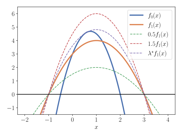
Two (non-convex) quadratic functions $f_0$ and $f_1$ for which $f_1(x)\leq 0$ implies $f_0(x)\leq 0$ for all $x\in\mathbb{R}$ . As stated by the S-lemma, we can thus find a value $\lambda\geq0$ such that $\lambda f_1(x)\geq f_0(x)$ for all $x\in\mathbb{R}$ .

As we can see (both from the figure and the fact that the signs of the $x^2$ terms are negative), both of the functions are concave. The roots of $f_1$ are $x=-1$ and $x=3$ , so $f_1(x)\leq0$ for any $x\leq-1$ or $x\geq3$ (notice that this is a non-convex, disjoint set). The roots of $f_0$ are $x=-0.5$ and $x=2$ ; as these are both located between the roots of $f_1$ , we have

\begin{equation*} f_1(x) \leq 0 \implies f_0(x) \leq 0 \quad \forall\,x\in\mathbb{R}. \end{equation*}

The S-lemma tells us that there is therefore some $\lambda\geq0$ such that

\begin{equation}\label{14} \lambda f_1(x) \geq f_0(x) \quad \forall\,x\in\mathbb{R}. \end{equation}

Multiplying $f_1$ by a non-negative scalar $\lambda$ does not change its roots or convexity, just scales its value, as can be seen in the figure above. We just need to find a $\lambda$ large enough so that $\eqref{14}$ is satisfied. From the figure, we see that $\lambda=1$ is too small while $\lambda=1.5$ is larger than needed. Solving the small SDP

\begin{equation*} \begin{aligned} \lambda^{\star} = \min_{\lambda} &\quad \lambda \\ \text{subject to} &\quad \lambda\geq0 \\ &\quad \lambda\begin{bmatrix} Q_1 & p_1 \\ p_1 & r_1 \end{bmatrix} \succcurlyeq \begin{bmatrix} Q_0 & p_0 \\ p_0 & r_0 \end{bmatrix} \end{aligned} \end{equation*}

with

\begin{align*} Q_0 &= -3, & p_0 &= 2.25, & r_0 &= 3, \\ Q_1 &= -1, & p_1 &= 1, & r_1 &= 3, \end{align*}

we find that the smallest $\lambda$ satisfying $\eqref{14}$ is $\lambda^\star\approx1.203$ . The code used to generate the figure and solve the SDP can be found here.

Proof of Strong Duality for the QC1QP

Let us now prove that strong duality holds for the inequality-constrained QC1QP; that is, the optimal values of the primal problem $\eqref{6}$ and dual problem $\eqref{7}$ are equal. By weak duality, we always have $d^\star\leq p^\star$ ; we will make use of the S-lemma to show that this inequality is in fact always tight.

From the primal problem, we know that

\begin{equation*} f_1(\bm{x}) \leq 0 \implies p^\star - f_0(\bm{x}) \leq 0 \quad \forall\,\bm{x}\in\mathbb{R}^n, \end{equation*}

since $p^\star\leq f_0(\bm{x})$ everywhere in the feasible set $\{\bm{x}\in\mathbb{R}^n\mid f_1(\bm{x})\leq0\}$ , by definition. Assuming the primal problem is strictly feasible (i.e., there exists some $\tilde{\bm{x}}\in\mathbb{R}^n$ such that $f_1(\tilde{\bm{x}})<0$ ), the S-lemma tells us that there exists some $\tilde{\lambda}\geq0$ satisfying

\begin{equation*} \tilde{\lambda}\begin{bmatrix} \bm{Q}_1 & \bm{p}_1 \\ \bm{p}_1^T & r_1 \end{bmatrix} \succcurlyeq \begin{bmatrix} -\bm{Q}_0 & -\bm{p}_0 \\ -\bm{p}_0^T & p^\star - r_0 \end{bmatrix}. \end{equation*}

Pre- and post-multiplying both sides of the above expression by

\begin{equation*} \begin{bmatrix} \bm{x} \\ 1 \end{bmatrix}^T \text{ and } \begin{bmatrix} \bm{x} \\ 1 \end{bmatrix}, \end{equation*}

respectively, and rearranging a little, we obtain

\begin{equation*} f_0(\bm{x}) + \tilde{\lambda}f_1(\bm{x}) \geq p^\star, \end{equation*}

which holds for all $\bm{x}\in\mathbb{R}^n$ . Noticing that the left hand side is equal to $\mathcal{L}(\bm{x},\tilde{\lambda})$ , we have

\begin{equation*} d(\tilde{\lambda}) = \inf_{\bm{x}}\mathcal{L}(\bm{x},\tilde{\lambda}) \geq p^\star. \end{equation*}

Recalling that

\begin{equation*} d^\star = \max_{\lambda\geq0}d(\lambda) \geq d(\tilde{\lambda}), \end{equation*}

we get $d^\star\geq p^\star$ . Combined with weak duality, this reveals that

\begin{equation*} d^\star \geq p^\star \geq d^\star, \end{equation*}

which of course implies $d^\star=p^\star$ , and therefore strong duality holds. This means that we can obtain the exact optimal value of the non-convex problem $\eqref{6}$ by instead solving the convex dual problem $\eqref{7}$ .

Equality Constraints

Consider instead the equality-constrained QC1QP

\begin{equation*} \begin{aligned} p^{\star} = \min_{\bm{x}} &\quad f_0(\bm{x}) \\ \text{subject to} &\quad f_1(\bm{x}) = 0, \end{aligned} \end{equation*}

which has dual

\begin{equation*} \begin{aligned} d^{\star} = \max_{\lambda,\gamma} &\quad \gamma \\ \text{subject to} &\quad \begin{bmatrix} \bm{Q}_0 & \bm{p}_0 \\ \bm{p}_0^T & r_0-\gamma \end{bmatrix} + \lambda\begin{bmatrix} \bm{Q}_1 & \bm{p}_1 \\ \bm{p}_1^T & r_1 \end{bmatrix} \succcurlyeq \bm{0}. \end{aligned} \end{equation*}

To prove strong duality holds, the standard S-lemma is no longer useful. Instead, we must turn to the S-lemma with equality, which is characterized in (Xia, Wang, & Sheu, 2014). It states the following:

S-Lemma with Equality

Suppose we have two quadratic functions $f_0(\bm{x})$ and $f_1(\bm{x})$ , defined as in $\eqref{2}$ , and assume certain technical conditions hold (see below). Then the implication

\begin{equation}\label{15} f_1(\bm{x}) = 0 \implies f_0(\bm{x}) \leq 0 \quad \forall\,\bm{x}\in\mathbb{R}^n \end{equation}

holds if and only if there exists some $\lambda\in\mathbb{R}$ such that

\begin{equation*} \lambda\begin{bmatrix} \bm{Q}_1 & \bm{p}_1 \\ \bm{p}_1^T & r_1 \end{bmatrix} \succcurlyeq \begin{bmatrix} \bm{Q}_0 & \bm{p}_0 \\ \bm{p}_0^T & r_0 \end{bmatrix}. \end{equation*}

Technical Conditions

Notice the similarity to the standard S-lemma, except that the left hand side of the implication $\eqref{15}$ is now an equality, $\lambda$ is unconstrained, and we have assumed some as-yet-unstated technical conditions. The full set of these conditions is provided in the paper linked above but is fairly complicated, so we will only state two sufficient ones here:

there exist points $\tilde{\bm{x}}_1,\tilde{\bm{x}}_2\in\mathbb{R}^n$ such that $f_1(\tilde{\bm{x}}_1)<0$ and $f_1(\tilde{\bm{x}}_2)>0$ (this is sometimes called the two-sided Slater’s condition) and $\bm{Q}_1\neq\bm{0}$ ; or
$\bm{Q}_1$ is strictly positive or negative definite.

The second of these conditions holds in the extremal eigenvalue problem we looked at previously, in which $\bm{Q}_1=\bm{1}_n\succ\bm{0}$ , with $\bm{1}_n$ denoting the $n\times n$ identity matrix. An example using the first condition is given in (Bishop, Gerding, & Tran-Thanh, 2020), where it is applied to an optimal learning problem.

Strong Duality

Assuming at least one of the sets of conditions required for the S-lemma with equality holds, the proof of strong duality for the equality-constrained QC1QP is essentially the same as that of the inequality-constrained case, so we won’t bother repeating it here (consider it an “exercise for the reader”). However, we will note that we can construct equality-constrained QC1QPs in which the technical conditions of the S-lemma with equality do not hold and as a consequence neither does strong duality. For example, consider the QC1QP

\begin{equation*} \begin{aligned} p^{\star} = \min_{\bm{x}\in\mathbb{R}^2} &\quad x_1x_2 \\ \text{subject to} &\quad x_2^2 = 0, \end{aligned} \end{equation*}

the constraint of which implies $x_2^\star=0$ and therefore the optimal value is $p^\star=0$ . The Lagrangian is

\begin{equation*} \mathcal{L}(\bm{x},\lambda) = x_1x_2 + \lambda x_2^2 = \bm{x}^T\underbrace{\begin{bmatrix} 0 & 1/2 \\ 1/2 & \lambda \end{bmatrix}}_{\tilde{\bm{Q}}(\lambda)}\bm{x}. \end{equation*}

However, since there is no value of $\lambda\in\mathbb{R}$ for which $\tilde{\bm{Q}}(\lambda)\succcurlyeq\bm{0}$ (one way to see this is to recall that the determinant of a positive semidefinite matrix must be non-negative, but $\mathrm{det}\,\tilde{\bm{Q}}(\lambda)=-1/4$ for all $\lambda$ ), the Lagrangian is unbounded below and the dual optimal value is thus $d^\star=-\infty$ , so there is an infinite duality gap.

Thanks to Connor Holmes for reading a draft of this post.